1D Flow
3Di offers the possibility to simulate 1D flow. This means that the computed flow velocity and discharge is averaged over the full cross-sectional area. Effects of variations in depth and width are included, but flow within a segment has only one direction. A 1D element can represent, for example, a channel, a hydraulic structure or a sewer pipe. The sections below describe how 3Di deals with the computations in 1D, some specific characteristics and the several types of 1D elements that are available.
1D Network
In the most abstract form, a 1D network can be viewed as a combination of nodes and lines. Such a network is translated to a grid, as described in Computational grid for 1D domain. The nodes and the connections have their own characteristics, like cross-section shapes, reference levels etc. Based on those, cross-sectional areas, storage and flow is computed.
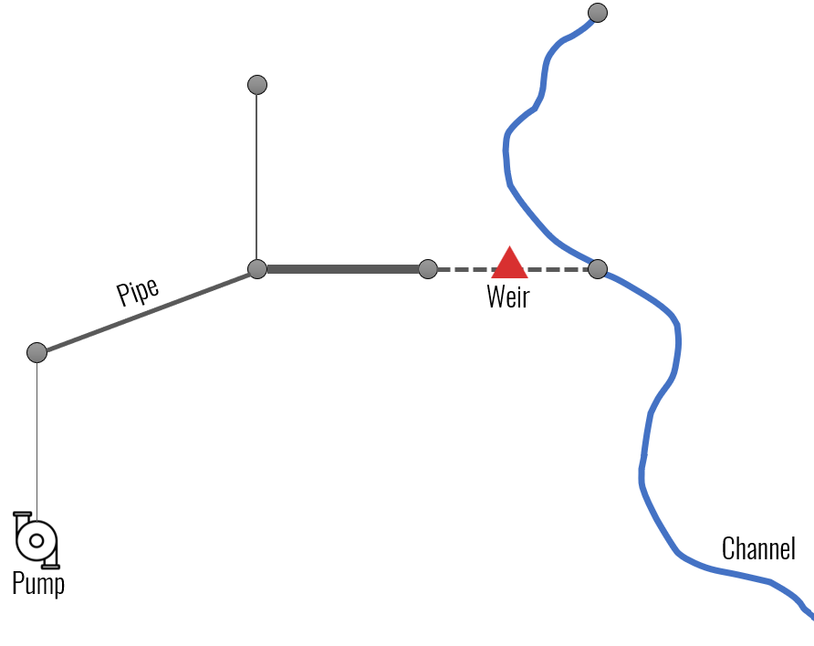
Fig. 66 Example of a 1D network
Cross-section shapes
Cross-sections in 1D can be open or closed. In open cross-sections, the width at the highest point in the cross-section definition is extrapolated straight up (red dashed lines in the figure below). In closed cross-sections, if the water level rises above the top of the cross-section, the volume and wet cross-sectional area remain the same, and the flow becomes pressurized. See Pressurized flow.
YZ cross-sections can be asymmetrical. Note that because 1D flow is width-averaged, only the width at each height is important; symmetrical and asymmetrical cross-section definitions will give the same results.
The table below gives an overview of the types of cross-section shapes available in 3Di.
Shape |
Value |
Description |
Open or closed |
|---|---|---|---|
Closed rectangle |
0 |
Rectangular cross-section |
Closed |
Open rectangle |
1 |
Rectangular cross-section |
Open |
Circle |
2 |
Circular cross-section |
Closed |
Egg |
3 |
Egg-shaped cross-section with the narrow end at the bottom. Width:height ratio is 1:1.5. |
Closed |
Tabulated rectangle |
5 |
Custom shape, with a width defined at each height. The width is used up to the next height/width pair without interpolation. |
Open if width at top > 0; Closed if width at top = 0 |
Tabulated trapezium |
6 |
Custom shape, with a width defined at each height. The widths are interpolated between height/width pairs. |
Open if width at top > 0; Closed if width at top = 0 |
YZ |
7 |
Custom shape, with a height (Z) defined at each distance (Y) across the channel or structure. |
Usually open, but can be closed when first YZ pair equals last YZ pair |
Inverted egg |
8 |
Egg-shaped cross-section with the narrow end at the top. Width:height ratio is 1:1.5. |
Closed |
Some examples are shown in the figures below.
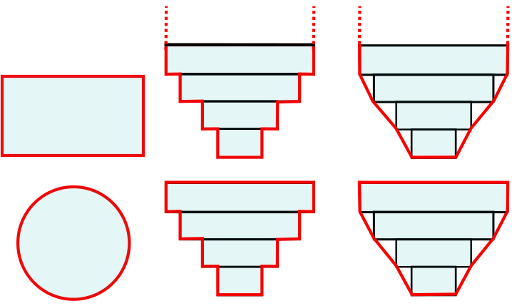
Fig. 67 Examples of cross-section shapes in 1D networks. Top row: Closed rectangle, Tabulated rectangle (open), Tabulated trapezium (open). Bottom row: Circle, Tabulated rectangle (closed), Tabulated trapezium (closed).
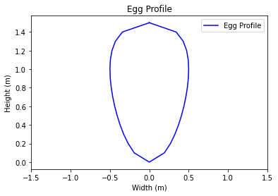
Fig. 68 Examples of cross-section shape ‘Egg’ in 1D networks. The ‘Inverted egg’ shape is the same, but upside-down.
1D momentum equation
The flow in 1D networks is computed using the equations of conservation of mass and momentum, more specifically the 1D depth-averaged shallow water equations. The momentum equation for 1D flow is:
In words; in 1D, 3Di takes inertia, advection, pressure gradients, bottom friction and wind shear stresses into account. This yields for all types of 1D network elements. However, there are some differences in the computation of advection and the effect of wind stress for specific 1D network This will be explained more elaborated, where these difference are relevant.
Friction in the 1D domain
3Di calculates the bottom friction or wall friction in the 1D-domain by integrating the shear stress over the cross-sectional area and over the length of the 1D element:
The conveyance factor is a measure of the flow capacity of a channel. The factor combines geometry and roughness information. There are two options to determine this factor. Both methods evaluate the friction based on the geometry and roughness of the section using either Chézy or Manning formulations for the roughness. In 3Di, friction types are distinguished as Chézy, Manning (for the 1st method) and Chézy with conveyance, Manning with conveyance (for the 2nd method).
Single section method
This method is suitable for closed, open, and semi-open sections. It assumes uniform roughness and velocity over the domain and therefore works best for relatively uniform cross-sections. This method considers the cross-section of the 1D element as a whole.
In the single section method, the conveyance factors are defined as:
with:
Conveyance method
The conveyance method (or compound section method), suitable for open sections only, allows for variations in the cross-flow direction. This method divides the channel cross-section into several sub-sections depending on the channel’s depth. This way, the variations in velocity related to the depth and roughness of the channel is properly taken into consideration.
The conveyance factor considers the depth variations in the different depth sections. The conveyance factor reflects the transport capacity of the channel. Assuming uniformity of the ratio between wetted perimeter and cross-sectional area, in applications with strong depth variations over the cross-section, underestimates the flow capacity. The conveyance method divides the channel cross-section into several sub-sections. In this method, the total conveyance factor of the section is the sum of each sub-section’s conveyance factor. In 3Di, the separation lines between the sub-sections are considered vertical .
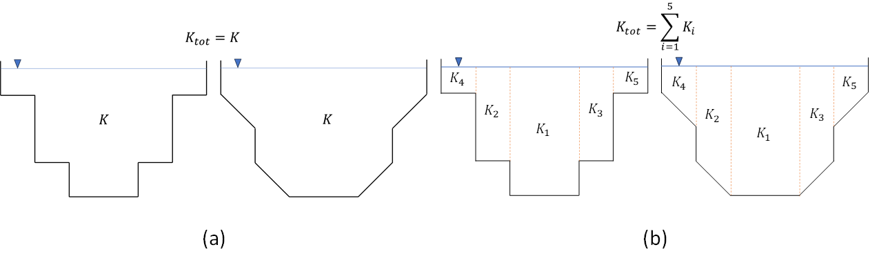
Fig. 69 Single Section Method vs Compound Section (Conveyance) Method
Pressurized flow
In 1D elements with closed cross-sections flow may become pressurized. The way 3Di deals with this is similar to how 3Di deals with the non-lineair relations in 2D cells (e.g. between volume and water level). Subgrid method allows 2D cells to be be dry, wet or partly wet, creating a non-lineair volume-water level relation. This was solved with a highly efficient method. However, there are some requirements for such system to be solved. one of these requirements is violated when the surface area decreases for increasing water levels, as in pipes that are more than half full (see the Figure below). Therefore, a new method had to be introduced to solve such a non-linear system of equations. This method is based on the so-called nested Newton method (cite:t:`Casulli2013).

Fig. 70 Examples of cross-sectional areas. An open and closed cross-sectional area
Because 3Di uses this method, not only flooding and drying is automatically accounted for, but also pressurized flow can be taken into account. One of the advantages is that from the moment the pipe is full (and the volume can no longer increase), the water level can still rise and the same flow equations are still valid. From this point forward, the ‘water level’ in the pipe represents a pressure. This makes 3Di calculations very stable in transitions between pressurized and non-pressurized flow, without the need for Preissmann slots or other workarounds.
Channels, culverts and pipes
Flow through channels, culverts and pipes is calculated with the 1D momentum equation.
The Channel, Culvert or Pipe in the schematisation is converted to multiple flowlines in the computational grid, see Calculation point distance.
Channels, culverts and pipes can exchange with the 2D domain (see 1D2D Exchange). The figure below illustrates this for a channel network.
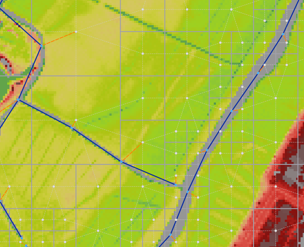
Fig. 71 Example network of connected channel sections and 2D quadtree with channel sections in blue, 1D2D connections in orange and the 2D quadtree in gray
The difference between channels, culverts and pipes is the way the inputs are specified (see 1D Objects). Culverts and pipes have the same cross-section along their whole length, while channels can have variable cross-sections. For culverts and pipes, the bottom level is specified only at the start and end (as invert levels), and are linearly interpolated from start to end. For channels, the bottom levels can be defined at multiple locations along the length of the channel.
Channels will generally have open cross-sections, but 3Di allows to assign closed cross-sections to channels, effectively making the channel a pipe. Inversely, pipes and culverts will generally have closed cross-sections, but 3Di allows to assign open cross-sections to pipes and culverts, effectively making them a channel.
Culverts can connect parts of 1D networks and allow flow under roads or other obstacles. In contrast to Weirs and Orifices, the flow behaviour in a culvert is assumed to be determined by shape and much less dominated by entrance losses. Culverts can be used for longer sections of pipe-like structures and do not have to be straight. Shorter, straight culverts are best modelled as an orifice. The energy loss caused by the change in flow velocity at the entrance and exit of culverts are accounted for in the 1D momentum equation. Any additional energy loss can be accounted for using the discharge coefficients, see Culvert.
Weirs and Orifices
Weirs are generally used to maintain and control the water level. Orifices connect two parts of channel networks. Both structures force the flow to converge strongly at the entrance and to diverge behind the structure. At the converging part of the flow, the assumption of conservation of momentum in 1D is invalid. Locally at the structure, conservation of energy is much more suited. The formulations for the flow over the weir and through the orifice are therefore based on Bernoulli’s principle. The computations of the flow of both structures follow the same reasoning. In the explanation below, the focus is on an open water rectangular weir, but similar steps are taken for structures with different open/closed cross-sections.
For a weir in open water the energy head balance reads:
where \(h\) is the local water depth, \(u\) the local cross-sectionally averaged velocity, \(g\) the gravitational acceleration and \(a\) the height of the crest. The sub-scripts refer to the flow domains, indicated in the figure below.
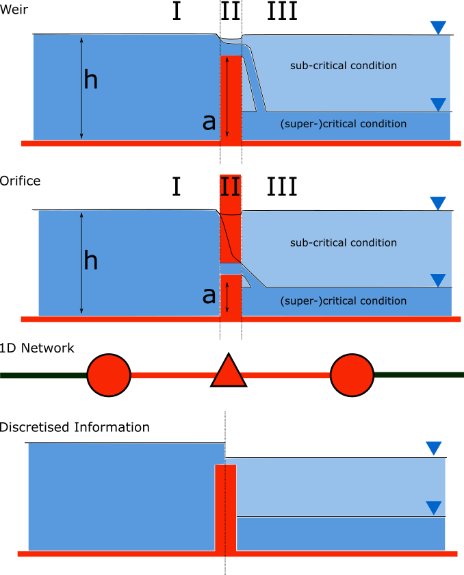
Fig. 72 Illustration of short crested weir and orifice under sub- and (super-)critical conditions; a simplified view of the 1D network and a sketch of the available discretized information.
In case of structures with closed profiles, in the equation of the energy balance \(h\) is not the water depth, but the energy height. For structures having closed profiles, the transition of water depth to energy height is automatically taken care of in case the area fills with water.
For robustness, 3Di schematizes structures as connections between two nodes, as can be seen in the third panel of the figure. This assumption implies that the water level on the location of the structure is unknown. To compute accurately the discharge over the structure, a difference is made between long crested and short crested structures. Both resulting formulations are based on Bernoulli’s principle, but for long crested structures, frictional losses are computed separately. The methods to resolve the flow over these structures, ensures numerical stability without time step dependence.
Short crested
The discharge over the structure is computed based on the effective cross-sectional area \(A_{eff}\) and the velocity over the structure \(u_{II}\). Two states of the flow can occur over the structure: sub- and (super)-critical flow. For both states, different assumptions are valid. However, for both states it is assumed that \(u_I\) is negligible compared to \(u_{II}\).
In case of (super-)critical flow, the downstream waterlevel does not affect the flow over the structure, as is the case under sub-critical conditions. The fourth panel of the figure shows the information known in a discretized world. In case the flow is critical, the water depth at the crest can be determined using the upstream waterlevel and the definition for critical flow:
The critical velocity over the structure is given by:
\(C_1\) is a loss coefficient, which can be set depending on the type and the shape of the structure itself and the entrance. The effective cross-sectional area is in this case based on the critical water depth. For a simple rectangular cross-section:
In which \(C_2\) is a loss coefficient due to contraction of the flow. For the total discharge in 3Di, the discharge under free flowing conditions is computed as:
Note, that the coefficients \(C_1\) and \(C_2\) are combined is the general discharge coefficient \(C\), which can be set by the user.
In case of sub-critical flows, the waterlevel downstream of the structure is important. Under these conditions the flow velocity over the structure is:
To determine the depth at the crest, it is assumed that the waterlevel at the crest is equal to the waterlevel downstream. Based on that assumption, the effective cross-section becomes:
Combining these equations, results in the discharge formulation.
Broad crested
For longer structures, frictional effects can become important. For the so-called broad-crested weirs and orifices an extra loss term is added to Bernoulli’s equation (the term is added to the right-hand side of the energy head balance equation at the top of this section). The extra head loss due to friction \(\Delta h_F\) is computed as:
where \(c_f\) is the dimensionless friction coefficient, \(L\) the length of the structure and \(R\) is the hydraulic radius on top of the weir. The dimensionless friction coefficient can be based on either the Manning or the Chézy formulation. The frictional losses scale with the length of the weir, therefore it is of importance that the structure length is correctly set. The computational core expects that this is the geometrical distance between the two connection nodes.
Pumps
Pumps in 3Di drain water from one location to another location, within the model domain (Pumpstation (with end node)) or out of the model domain (Pumpstation (without end node)). The behaviour of a pump is specified by defining the start and stop levels of the pump and the pump capacity, as illustrated in the figure below. See Pumpstation (with end node) and Pumpstation (without end node) for details on how to set these parameters.
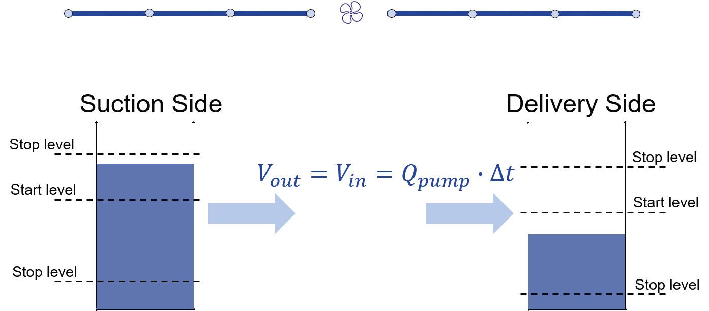
Fig. 73 Schematic display of a pump function
The pumped volume in the flow summary only includes the pumpstations without end nodes.
Pump capacities are often larger than the discharge to the pump, causing the pump to switch on and off frequently. This leads to strong fluctuations in water levels and pump discharge on the short term. Averaging this out, i.e. setting the pump capacity to the supply discharge, will make the simulation more balanced, with the same water system behaviour on longer time scales. This can be done by setting the Pump implicit ratio.
Pumps can be used in combination with controls. You can design a control that allows the water level at different or multiple locations determine the pumps behaviour, instead of purely local water levels. However, the local availability of water will always affect the pump capacity as well. As water that is not locally at the pump cannot be drained away. This is ensured by stopping the pump when the local water level is below the stop level. Your control affects the pumps’ behaviour, within the range of conditions for which the pump is designed.
Example
Given a controlled pump at location X with a stop and start level of 0.0 mNAP and 2 mNAP, respectively. The trigger for the control is the water level from location A. For higher waterlevels the pump capacity is increased. However, in case the water level at X is below 0.0 mNAP, but at A in a active range, the pump will stop. The pump can only become active again for waterlevels at X above 2.0 mNAP.