Tutorial 6: Analysing simulation results

Introduction

In this tutorial, we explore how you can analyse simulation results using the 3Di Modeller Interface. This tutorial is a bit longer than the previous tutorials. It has a number of sub-sections:

• Running the simulation

• Assessing the flood impact

• Why does the inundation occur?

• Quantification of the flood volume

• Applying measures

Case study

Our study is Langå, a small railway town located in central Denmark.

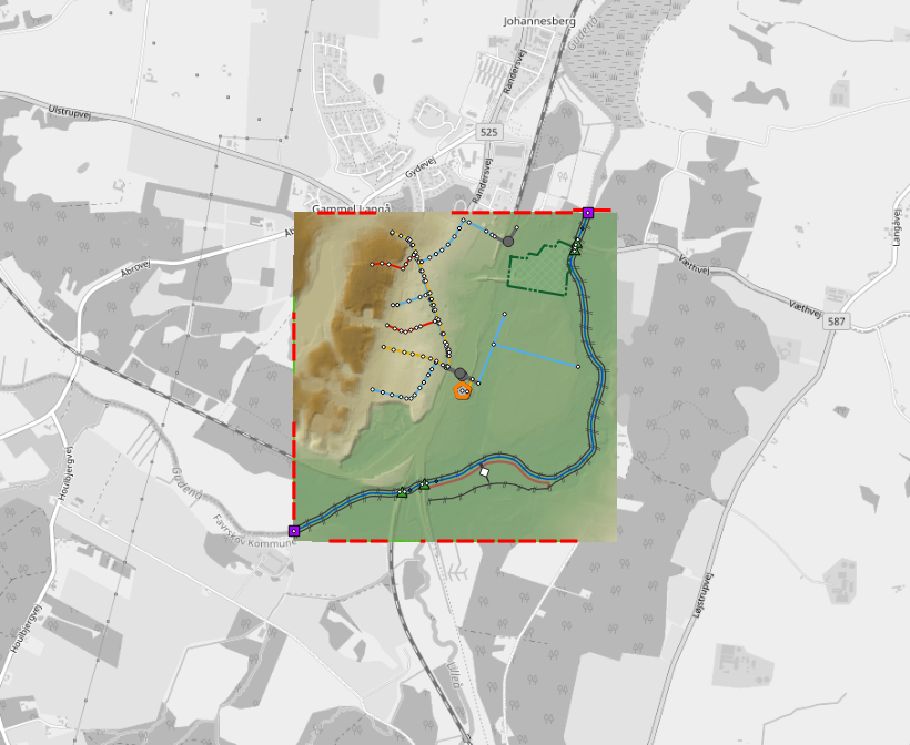
Langå is situated between raised agricultural lands to the west and the Gudena River to the east of the town. The urban area has a seperated sewer system. The sanitary sewer inclines towards a pumping station, and the stormwater sewer has two outlets close to the Gudena River.

Several houses on the road Vaethvej (numbers 21-29) are vulnerable to flooding. Recently, the inhabitants living there have reported flood problems after a 40 mm rainfall event.

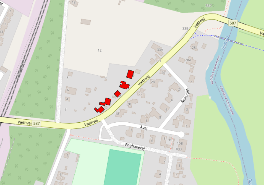
Now the municipality wants to reproduce this inundation with a hydrodynamic model, to gain insight in the flood properties such as flood extent, flood volume, and flood duration. The municipality also wants to know where the flood water originates from. These insights will help the municipal government to design measures to reduce the flood risk.

Note

While this tutorial represents a real-world area, it is important to note that some processes have been simplified for the purpose of this tutorial and that the situations described in it are hypothetical.

Learning objectives

You will learn the following in this tutorial:

• Downloading simulation results

• Checking the flow summary

• Generaring a maximum inundation depth raster

• Analysing the flow pattern

• Finding the maximum inundation depth

• Plotting water levels

• Watershed delineation for a flooded area

• Calculating the flood volume

Preparation

Before you get started:

• Make sure you have a 3Di account. Please contact the Service desk if you need help with this.

• Install the 3Di Modeller Interface, see Install and update manual.

• Download the dataset for this tutorial here.

• Unzip the dataset for this tutorial and save the contents in your Downloads folder.

The dataset that you downloaded for this tutorial contains a 3Di schematisation, consisting of a Spatialite (.sqlite file) and a Digital Elevation Model (.tif file) for the place Langå. The DEM is located in the folder named “rasters”.

Running the simulation

We will go through a number of steps to run a simulation, to have results that we can analyse. These steps should mostly be familiar if you have already done one or more of the previous tutorials.

Creating a new schematisation

The first step is to create a new Schematisation:

1. Open the 3Di Modeller Interface.

2. Click the 3Di Models and Simulations. You should now see the 3Di Models and Simulations panel. If this is the first time you use the 3Di Models and Simulation panel, you will need to go through some steps to set it up.

3. In the Schematisation section of the 3Di Models and Simulations panel, click New. The New schematisation wizard is shown.

4. Fill in a schematisation name, such as ‘Tutorial analysing simulation results Langaa <your_name>’. Select the organisation you want to be the owner of the new schematisation (most users have rights for only one organisation). Tags are optional, you can leave this field empty for now. Since you will use a pre-built schematisation, select the Choose file option. Select the schematisation file Demo model Langaa.sqlite from your Downloads folder.

5. Click Create schematisation. A popup message will tell you that the schematisation was created successfully.

Uploading the schematisation

We will now upload the schematisation as a first Revision and process it into a 3Di Model. All these steps are covered by the upload wizard.

1. Click the upload button in the 3Di Models and Simulations panel.

2. In the dialog box that has appeared, click New upload and click Next.

3. Click Check schematisation. This will check your schematisation for any errors that would make it impossible to generate a valid 3Di model and simulation template. It should not produce any errors, warnings or info level messages. Click Next.

4. Fill in a commit message. This is a short description of the changes you have made relative to the previous revision. As this is the first revision of this schematisation, you can provide a short description of what you upload. For example: “Langå schematision without changes”.

5. Click Start upload. Check whether the upload is successful and the schematisation is successfully processed into a 3Di model.

Viewing the schematisation

We will load the schematisation in the 3Di Modeller Interface to view it. Later in this tutorial we will also make some modifications. The schematisation can be loaded by following these steps:

1. In the 3Di Schematisation Editor toolbar, click the Load from Spatialite button.

2. Double-click the name of the schematisation you want to load.

3. Add a background map from OpenStreetMap by clicking Web in the Main Menu > Quick Map Services > OSM > OSM Standard.

4. In the Layers panel, reorder the layers such that the OpenStreetMap layer is below the 3Di schematisation.

You should now see the DEM around Langå.

Running a simulation

We will now start a simulation with the 3Di model you have created in the 3Di Modeller Interface:

1. In the 3Di Models and Simulations panel, click Simulate > New simulation.

2. Select your model and simulation template and click Next. A dialog box opens with several options for your simulation.

3. Check the box Include precipitation. Keep Include initial conditions and Include boundary conditions checked. Click Next.

4. Give your simulation a name, e.g. Demo Langaa 40mm constant rainfall in 1 hour. Click Next.

5. Set the duration of your simulation to 4 hours. Click Next.

6. Accept the Boundary conditions as they are by clicking Next.

7. Accept the Initial conditions as they are by clicking Next.

8. Fill in the following parameters for Precipitation and then click Next.

   • Type of precipitation: choose Constant

   • Start after: 1 hrs

   • Stops after: 2 hrs

   • Intensity: 40 mm/h

9. Accept the simulation settings as they are by clicking Next.

10. Check the summary of your simulation and click Add to queue.

Your simulation will start as soon as a calculation node is available for your organisation. Note: the number of available calculation nodes depends on your 3Di subscription.

In the 3Di Models and Simulations panel, click Simulate. An overview is given of all running simulations for your organisation(s). Here you can follow the progress of your simulation.

You may also follow the simulation in 3Di Live.

Assessing the flood impact

Now that we have ran the simulation, we can start analysing. Our first step will be to assess the flood impact: where does it flood, with what depths and for how long?

Downloading the simulation results

We will now download the results of your simulation to your working directory which is a local folder:

1. In the 3Di Models and Simulations panel, click Results .

2. Select your simulation and click Download. A download progress bar now appears. This progress bar colors green when the downloading of your simulation results is finished.

Note

The simulation results are saved in your 3Di working directory. To open this folder, click on the name of the schematisation in the 3Di Models & Simulations panel.

Opening the simulation results

Our next step is to load the simulation results in the 3Di Modeller Interface.

1. In the 3Di Results Analysis toolbar, click the 3Di Results Manager button . The 3Di Results Manager panel now opens.

2. In the 3Di Results Manager panel, click on the Add 3Di grids or results button.

3. Select your simulation and click Load simulation results, or double click the name of your simulation.

Now your simulations results are loaded in the 3Di Modeller Interface and shown in the Layers panel.

Checking the flow summary

As a first step of gaining insight in the simulation, we will check out the Flow summary.

1. In the 3Di Models & Simulations panel, click on the name of the schematisation to open the folder where the simulation results are downloaded to.

2. Open the document flow_summary.json.

First, we will check if the total rainfall volume in the flow_summary.json matches the rainfall event (40mm in one hour). To be able to calculate this, we need to know the surface area of the model.

1. In the 3Di Modeller Interface, in the Layers panel, right-click on the layer Digital elevation model > Properties.

2. Under the Information tab, in the Information from provider section, you can find the width and height (in pixels), and pixel size (in meters). Combine this information to calculate the area of the DEM and the total rainfall volume. Does it correspond with the total rain on 2D reported in the Flow summary?

Note

The 3Di Model in this example is atypical in that it is perfectly rectangular. All pixels in the DEM have a value. Most 3Di Models have a boundary that follows hydrogical watershed boundaries. DEM pixels outside of these boundaries are “no data” pixels. In such a case, the method used here for calculating the surface area of the model does not work. Instead, use the QGIS Processing Algorithm “Zonal statics”, with an input polygon that covers the entire model domain, and choose “Count” as one of the statistics to calculate.

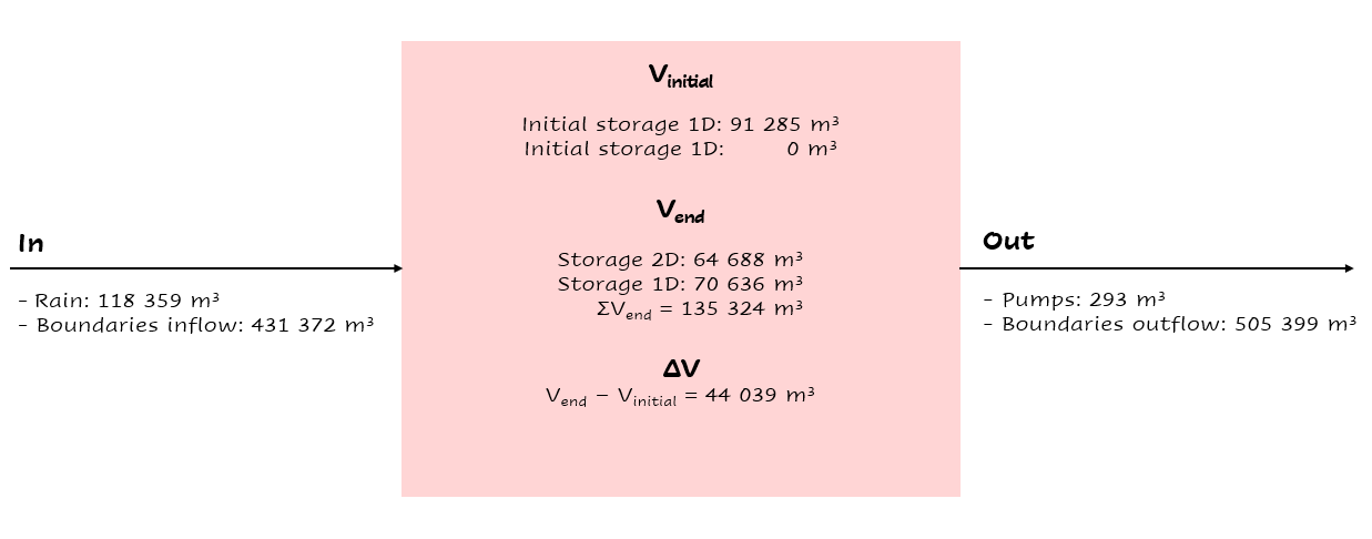
Secondly, you are going to make a volume balance to better understand the functioning of the model.

1. Draw your own water balance, indicating the inflow, volume change, and outflow. Alternatively, you can use the empty balance below:

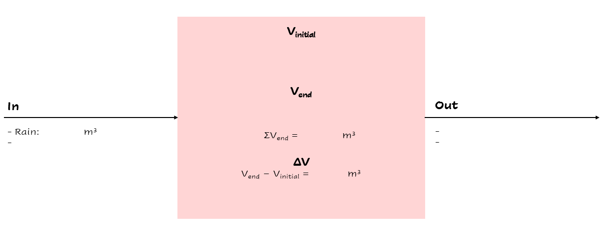
1. Now fill in the water balance with the numbers you find in the flow summary. Check the water balance yourself; do the numbers add up? Does the difference correspond with the volume error reported in the flow summary?

The filled-in water balance can be found below. Note that the exact numbers may differ, as changes are sometimes made to the tutorial model.

Generating the maximum water depth raster

In this step, we are going generate a maximum inundation depth map.

1. Open the Processing Toolbox (Main Menu > Processing > Toolbox).

2. In the Processing Toolbox panel, click on 3Di > Post-process results > then double click Maximum water depth / level raster.

Now a new panel opens where we can define the settings for the maximum water depth raster that we are going to create.

1. Select your gridadmin.h5 file by clicking on the browse button and browse to your working directory folder (e.g. C:3Di_schematisations) > Demo model Langaa > revision 1 > results > Demo Langa 40mm constant rainfall in 1 hour > gridadmin.h5.

2. Select your simulation results file (results_3di.nc). This file is located in the same directory as the gridadmin.h5 file.

3. Select the DEM (Digital Elevation Model) by clicking on the browse button under DEM. Browse to your working directory > Demo model Langaa > work in progress > schematisation > rasters > Elevation_model_Langaa.tif.

4. Set the Interpolation mode to Interpolated water depth.

5. Set the destination file path for water depth/level raster by clicking the browse button. Browse to your working directory > Demo model Langaa > revision 1 > results.

6. Write the file name max_water_depth_interpolated.tif.

7. Click Run.

When finished, the raster will automaticaly appear in the Layers panel. Now we are going to add a basic styling to this raster.

1. In the Layers panel, double click the layer max_water_depth_interpolated. The Layer Properties window opens.

2. In the layer properties window, the Symbology tab (at the left side).

3. Set Render type to Singleband pseudocolor.

4. Set Color ramp/ to Blues.

5. Fill in 0.0 as Min value and 0.5 as Max value. These are units in meters.

We will now make all water depths between 0 and 1 cm transparent.

1. In the Transparency tab, under Custom transparency options, click the + button.

2. For From, fill in 0; for To, fill in 0.01.

3. Click OK.

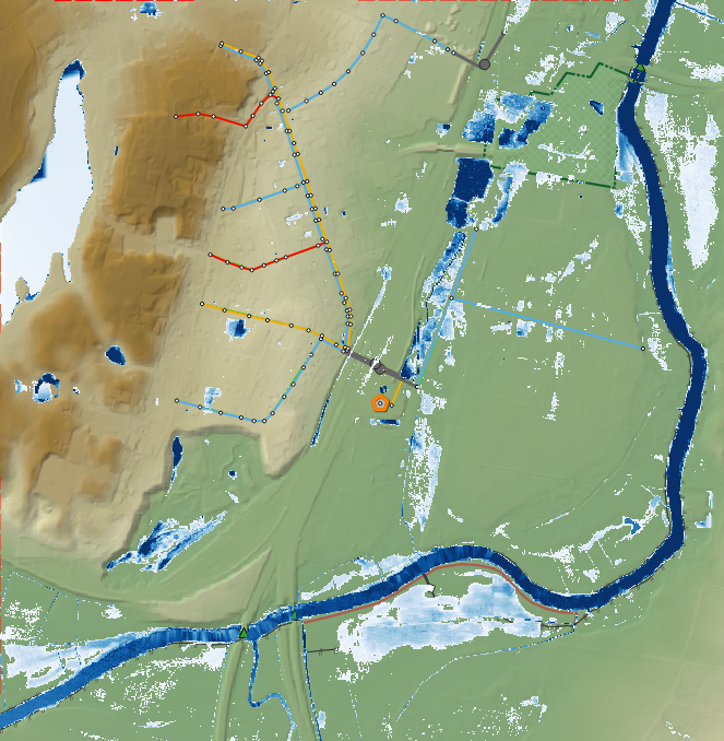
The result should look like this:

Finding the maximum inundation depth

We are going to use the Value Tool to view the inundation depth in our study area using the maximum water depth raster.

1. First, make sure the maximum water depth raster is visible. In the Layers panel, check the layer max_water_depth_interpolated.

2. In the Attributes Toolbar, click on the Value Tool button. Now the Value Tool panels opens.

3. Now zoom in to our study area; with your mouse, hoover over the inundated area. In the Value Tool panel, you can read the raster values, i.e. the maximum inundation depth. Find that the inundation is up to 75 cm.

How long does the inundation last?

The maximum water depth map gives insight in where the flooding occurs, but does not show when this happens. Plotting a time series of the water level will give this insight.

1. In the 3Di Result Analysis Toolbar, click on the Time series plotter icon. Now the 3Di Time series plotter panel opens.

2. In the 3Di Time series plotter panel, click on Pick nodes/cells.

3. Click on a 2D surface water node in the inundated area near Vaethvej 21-29. A graph is plotted for the selected 2D node. Note: make sure that in the upper right drop-down menu of the 3Di Time series plotter panel, the selected variable is Water level.

4. Look at the graph. When does the water level start rising? When does the peak occur and why? Why does the rate of rise decrease leading up to the peak? Is the decrease after the peak faster or slower than the increase? What does this graph tell you about the drainage situation at this location?

Note

If your subscription also includes the Scenario Archive, you can add a WMS layer of the water depth, and use the Temporal Controller to navigate through its time steps. This will give you additional insight in the progression of the flood through time. See the `Lizard documentation<https://docs.lizard.net/d_qgisplugin.html>`_ for more information.

Why does the inundation occur?

Now that we have established the impact and severity of the flooding, we will look into why it happens at this location. If we know where the water comes from, we know where we can add extra buffer capacity. If we know which routes the water follows, we may be able to change those routes. We may also be able to drain water from the area more quickly.

Analysing the flow pattern

We will start by visualising the flow pattern. Make sure you have added the results in the 3Di Results Manager.

1. In the 3Di Results Manager panel, click the icon.

In the Layers panel, the node, flowline and cell layers have been renamed to the variable that is visualised.

1. Toggle the Node and Cell layers (“Water level [m MSL]”) to invisible.

You now see the net cumulative discharge over the whole simulation for each flowline. You may move the time slider in the Temporal Controller at the top of the screen to view the results for earlier moments in the simulation. In the 3Di Results Manager panel, you can also change the visualised variable to Discharge to get a snapshot of the situation at the time step you have navigated to in the Temporal Controller.

1. Zoom out from the Vaethvej a bit. Can you see the flow route(s) the water follows to flow to our problem area? By which route(s) does the water leave?

Another way to analyse the flow pattern is by using the 3Di Results Aggregation tool.

1. Switch off the flow visualisation by clicking the Eye icon in the 3Di Results Manager panel.

2. Click 3Di Result Aggregation in the 3Di Results Analysis toolbar. A pop-up screen will appear.

3. In the Input tab, the simulation result is selected automatically.

4. Under Preset, select Flow pattern. If you are interested, you can play around with the other presets options later. Click OK. The flow pattern will now be derived and thre resulting layer will be added to the project.

Note

The layer Flow pattern (nodes) shows an arrow for each calculation node; the layer Flow pattern (nodes)_resampled_nodes is based on the same data, but spatial interpolation has been applied to downsample the data to the resolution of the smallest calculation cell in the model.

1. In the Layers panel, right-click the group 3Di Results > Zoom to Group. Look at the elevation map and the flow pattern; note that the water flows from the higher areas towards the lower areas and a large part eventually ends up in the river.

The result should like like this:

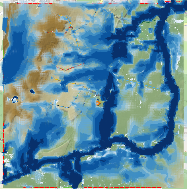
1. You can zoom in on the flow pattern to discern the individual arrows. As you can see, the direction of the arrow indicates the direction of the flow. The colour of the arrow is scaled with the discharge.

Watershed delineation for a flooded area

Another quick way to find out where the flood water comes from is using the Watershed Tool. The Watershed Tool allows you to determine the upstream and downstream catchment at any point or area.

1. First, we have to make sure the maximum water depth raster is visible and the results from the previous step are hidden. In the Layers panel, check the layer max_water_depth_interpolated. In the group 3Di Results > {name of your 3Di Model}, uncheck the group Result aggregation outputs.

2. In the group 3Di Results > {name of your 3Di Model} > Computational grid, make sure all the layers and the group itself are checked, so that the nodes are visible.

3. Now, open the Watershed tool in the 3Di Results Analysis toolbar.

4. In the Watershed tool panel, define the Input: select your simulations results under 3Di results.

5. Leave the Settings as they are.

6. In the section Target nodes, click Click on canvas to activate the map tool. On the map canvas, click on a node in the inundated area near Vaethvej 21-29.

The tool automatically calculates the upstream catchment area for the nodes that you selected. By choosing Clear results, the catchment will disappear and you can choose different nodes to derive the upstream catchment for.

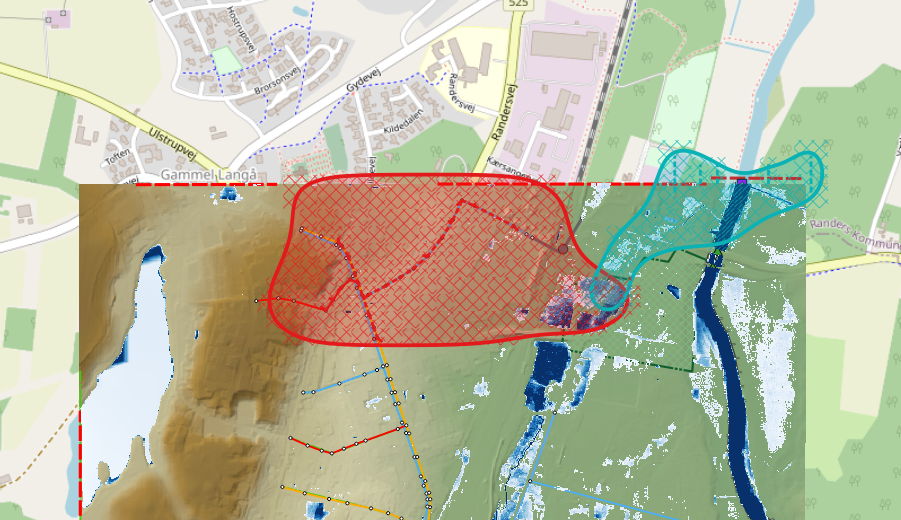
1. In the Output section, check the Downstream option and uncheck the Upstream option. The result gives us a indication of how the flood volume is drained during and after the event.

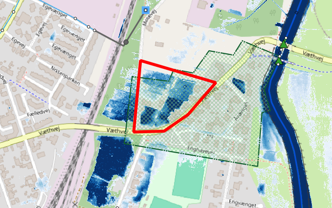
The upstream and downstream areas for Vaethvej 21-29 should look like this:

1. Using the methods outlined above, can you identify a suitable location for a flood retention basin?

Tip

Use a satellite imagery background map to help you assess the suitability of the chosen location. Click Main Menu > Web > QuickMapServices > Search QMS. In the QMS panel that opens, search for “Satellite”. Choose the option you like, e.g. Google, Esri, or Bing Maps.

Quantification of the flood volume

Now that we know where additional storage or buffer capacity would be helpful, we need to estimate how much storage is needed, so that we can use the correct dimensions in the design of our measure.

Calculating the flood volume

To determine the flood volume in our study area, we are going to use the Water balance tool. This tool calculates a water balance for each time step for a given area. We will start by creating a polygon layer that defines the area we want to make a water balance for.

1. Click Main Menu > Layer > Create new layer > New Temporary Scratch Layer. Fill in the following values:

   • Layer name: “Flood risk area”

     • Geometry type: Polygon

     • CRS: EPSG:4094 - ETRS89 / DKTM2

     • You do not have to add any fields

     • Click OK

2. The new layer is added to the project in edit mode. Click Add Polygon Feature in the main toolbar.

3. Draw a polygon around the Vaethvej 21-29 area, stop the editing session and save your edits. The polygon should look more or less like this:

1. Click the Water balance tool button in the 3Di Results Analysis toolbar.

2. Choose Select polygon and click on the polygon. Choose Flood prone area in the context menu. The tool will now automatically calculate and visualize the water balance for this area.

3. In the water balance plot, you can either show discharge (m³/s) or volumes (cumulative discharge, m³). The tool is automatically set to discharge. Now change to volume by using the dropdown menu and choose the m³ cumulative option.

4. In the graph, the cumulative volumes of water for flows are displayed. At the right side, you can activate and deactivate different the flows. Hover over the different components to see which ones are indicated in the graph.

The main component that is of interest in this question is 2D flow. Notice that the graph displays both a positive and negative cumulative 2D Flow. The positive 2D flow indicates flow into the polygon, the negative 2D flow indicates flow out of the polygon. The net 2D flow (change in storage) is represented by the dotted red line, representing the volume change 2D. Use your mouse to zoom in on the y-axis. You can check the net 2D volume change at the end of the simulation, which should be around 2000 m³.

1. What is the total (gross) inflow into the polygon?

Applying measures

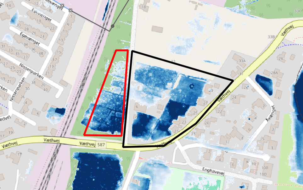
The last step is to include the new retention area in the model, to see if it works as intended. Based on our analysis and the suitability of the terrain, the following location is chosen as retention area:

Drawing the retention area polygon

1. Create a new scratch layer, in the same way as you did in tut6_calc_flood_volume. Name it “Retention area”.

2. Draw the new retention area on the map.

3. Make sure the layer “Retention area” is selected in the Layers panel.

4. Click Main Menu > View > Panels > Layer styling to open the Layer Styling panel.

5. In the Layer Styling panel, go to the Labels tab and set it to Single labels

6. In the Value input, type round($area). Now click anywhere outside that input field. The Retention area polygon should now be labelled with its surface area (in square meters).

7. In the sub-tab Buffer, check the box Draw text buffer to make the label easier to read.

8. How deep must the retention area be so that it can contain all the water that flows into the flood prone area at Vaethvej 21-29?

9. Use the Value Tool to find out what the current elevation is within the new retention area. What should be the new elevation of the bottom of the retention area?

Editing the DEM

We will now use this polygon to edit the DEM, so that we can assess the effect of the new retention area.

1. Open the Processing Toolbox (Main Menu > Processing > Toolbox).

2. In the search bar, type “Rasterize”

3. Open the Processing Algorithm “GDAL > Vector Conversion > Rasterize (overwrite with fixed value)”

4. Fill in the following parameters:

   • Input vector layer: “Retention area”

   • Input raster layer: “Digital Elevation Model [m MSL]”

   • A fixed value to burn: fill in the new elevation that you have calculated in the previous step

5. Click OK and wait for the processing algorithm to finish.

6. When the processing algorithm is finished, use the Value Tool to check if the new value has been burned into the DEM correctly.

Running a simulation with the edited DEM

You can now repeat the steps you have done earlier in this tutorial to check if the measure has been effective.

• Uploading the schematisation

• Running a simulation

• Assessing the flood impact

Has this measure solved the whole flood problem for Vaethvej 21-29? If not, what additional measures can be taken?

Congratulations

Well done! You have finished the tutorial Analysing simulation results!

If you would like to learn more about the tools available for analysing your 3Di simulation results, check out the Analysing results in the 3Di Modeller Interface section of the 3Di Modeller Interface User Manual.