2D Objects
2D objects are calculated in the 2D domain. There are several 2D objects:
2D Boundary Condition
Boundary condition for 2D model edge. Boundary conditions are crucial in hydraulic modeling because they define the interactions between the modeled area and its surroundings. They help simulate how water flows into or out of the simulation domain and how different types of forces, like inflows, outflows, water levels, or water velocities, are accounted for at the edges of the simulated region.
Geometry
Line
Geometry requirements:
2D boundary condition line can only touch boundary computational cells. These are defined as cells having at least one side that does not share an edge with another computational cell. This is often a cell at the outer edge of the model domain. It is also possible to schematise 2D boundaries on an inner edge of the model domain, i.e. if there is a NODATA hole in the DEM.
2D boundary condition lines must intersect with one or more computational cells.
When multiple computational cells are touched by the 2D boundary condition line, it is essential that these cells align either vertically or horizontally. Diagonal alignment is not permitted.
All cells intersected by a 2D boundary condition line must have the same size, i.e. do not use grid refinement at the location of a 2D boundary condition.
Tip
When experiencing difficulties adding 2D boundary conditions, generate the computational grid locally using Computational grid from schematisation. This helps you see where the 2D boundary condition line is located relative to the computational cells.
Attributes
Field name |
Type |
Mandatory |
Units |
Description |
|---|---|---|---|---|
id |
integer |
Yes |
- |
Unique identifier |
display_name |
text |
Yes |
- |
Name field, no constraints |
boundary_type |
text |
Yes |
- |
Sets the type to Waterlevel, Velocity, Discharge, Sommerfeld, Groundwater level or Groundwater discharge |
timeseries |
text |
Yes |
[minutes since start of simulation],[m | m/s | m³/s] |
Timeseries of water levels, flow velocities, discharges or water level gradients to be forced on the model boundary |
Time series
Format the time series as Comma Separated Values (CSV), with the time (in minutes since the start of the simulation) in the first column and the value (units dependent on the boundary type) in the second column. For example:
0,145.20
15,145.23
30,145.35
45,145.38
60,145.15
The time series string cannot contain any spaces or empty rows
The boundary condition time series is stored in the simulation template and is not part of the 3Di model itself. It can be overridden when starting a new simulation, without the need to create a new revision of the schematisation.
The time unit in the 2D boundary condition table in the schematisation is minutes, while the 3Di API expects this input in seconds. A conversion is applied when the reading the data from the schematisation. If you upload a CSV file with 1D boundary condition time series via the simulation wizard, you can choose the time unit (see Boundary conditions)
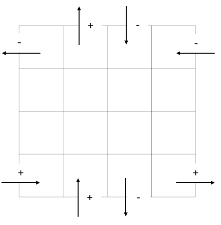
For boundary types velocity (2), discharge (3) and Sommerfeld (5), the sign of the input values determine the flow direction (see the figure below). If a 2D discharge or velocity boundary condition is placed at the eastern or northern edge of the model domain, and you want water to flow in (from east to west or from north to south), the values must be negative; if it is placed at the western or southern edge, the values must be positive to make the water flow in. For the Sommerfeld boundary, a positive value (gradient) means that the water level at the western/southern side is lower than the water level at the eastern/northern side, i.e. if placed at the east or north, this will result in boundary inflow and if placed at the west or south, it will result in boundary outflow.
Discharge values are applied to all intersected flowlines. So if the value is 5 m³/s and the geometry of the 2D boundary condition intersects 3 flowlines, the total in- or outflow will be 15 m³/s. Generate the computational grid locally using Computational grid from schematisation to determine how many flowlines are intersected.
The time series must cover the entire simulation period.
The time series values are interpolated between the defined times
In case of multiple boundaries in 1 model: make sure they all have the same number of time series rows with the same temporal interval.
When editing the time series field in using SQL (sqlite dialect), use
char(10)as line separator. The example time series shown above would look like this:"0,145.20"||char(10)||"15,145.23"||char(10)||"30,145.35"||char(10)||"45,145.38"||char(10)||"60,145.15"
2D Lateral
Lateral discharge for 2D cell.
Geometry
Point
Attributes
Field name |
Type |
Mandatory |
Units |
Description |
|---|---|---|---|---|
id |
integer |
Yes |
- |
Unique identifier |
type |
text |
Yes |
- |
Type of 2D lateral: Surface |
timeseries |
text |
Yes |
[minutes since start of simulation],[m³/s] |
Timeseries of lateral discharges to be added to the specified location |
Notes for modellers
Time series
Format the time series as Comma Separated Values (CSV), with the time (in minutes since the start of the simulation) in the first column and the value (m³/s) in the second column. For example:
0,0.2
15,10.0
30,20.0
45,7.5
60,0.0
The time series string cannot contain any spaces or empty rows
Linear obstacle
Line with fixed crest level that overrides DEM values at edges of computational cells when calculating the cross-section between cells.
Geometry
Line
Attributes
Field name |
Type |
Mandatory |
Units |
Description |
|---|---|---|---|---|
fid |
integer |
Yes |
- |
Unique identifier |
id |
integer |
Yes |
- |
Unique identifier |
code |
text |
No |
- |
Name field, no constraints |
crest_level |
decimal number |
No |
m MSL |
Lowest point of the obstacle |
Grid refinement
Lines that determine local 2D calculation grid refinement.
Geometry
Line
Attributes
Field name |
Type |
Mandatory |
Units |
Description |
|---|---|---|---|---|
id |
integer |
Yes |
- |
Unique identifier |
display_name |
text |
Yes |
- |
Name field, no constraints |
code |
text |
Yes |
- |
Name field, no constraints |
refinement_level |
integer |
Yes |
- |
The maximum number of grid-refinement levels. See Computational grid for more details. |
Grid refinement area
Polygons that determine local 2D calculation grid refinement.
Geometry
Polygon
Attributes
Field name |
Type |
Mandatory |
Units |
Description |
|---|---|---|---|---|
id |
integer |
Yes |
- |
Unique identifier |
display_name |
text |
Yes |
- |
Name field, no constraints |
code |
text |
Yes |
- |
Name field, no constraints |
refinement_level |
integer |
Yes |
- |
The maximum number of grid-refinement levels. See Computational grid for more details. |
DEM average area
Polygons that determine in which cells DEM averaging should be applied.
Geometry
Polygon
Attributes
Field name |
Type |
Mandatory |
Units |
Description |
|---|---|---|---|---|
id |
integer |
Yes |
- |
Unique identifier |
Windshielding
Windshielding reduces the wind shear on open water.
Geometry
No geometry
Attributes
Field name |
Type |
Mandatory |
Units |
Description |
|---|---|---|---|---|
id |
integer |
Yes |
- |
Unique identifier |
channel_id |
integer |
No |
- |
ID of the channel |
north |
decimal number |
No |
- |
The amount of wind being shielded from the north. |
northeast |
decimal number |
No |
- |
The amount of wind being shielded from the northeast . |
east |
decimal number |
No |
- |
The amount of wind being shielded from the east. |
southeast |
decimal number |
No |
- |
The amount of wind being shielded from the southeast. |
south |
decimal number |
No |
- |
The amount of wind being shielded from the south. |
southwest |
decimal number |
No |
- |
The amount of wind being shielded from the southwest. |
west |
decimal number |
No |
- |
The amount of wind being shielded from the west. |
northwest |
decimal number |
No |
- |
The amount of wind being shielded from the northwest. |